INTRODUCTION
This experiment uses a ramp and a low-friction cart. As the cart rolls down a ramp, it builds up speed – accelerates. Using a photogate, we will investigate the pattern by which the speed (velocity) increases. In the process we will learn more about some of the features of Logger Pro software.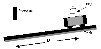
Figure 1
OBJECTIVES
* Collect data as a cart rolls
different distances down an inclined plane
* Analyze the graph of time (Dt) vs. distance (D) for the cart
* Analyze the graph of velocity (v) vs. distance for the cart
* Analyze the graph of time (Dt) vs. distance (D) for the cart
* Analyze the graph of velocity (v) vs. distance for the cart
MATERIALS
computer
Vernier Photogate
Vernier computer interface
Vernier Dynamics System
Logger Pro
Flag cut from Index Card
Vernier Photogate
Vernier computer interface
Vernier Dynamics System
Logger Pro
Flag cut from Index Card
PRELIMINARY QUESTIONS
1. Sketch your prediction for the speed vs. distance graph as the cart rolls down the ramp. Describe in words what this graph means.2. How would your predicted graph change if you changed the angle of the incline? Explain.
PROCEDURE
1. Set up the equipment as illustrated in Figure 1. Make the “flag” from an index card, making the top 2.0 cm wide (d). Tape it to the side of the cart.2. Adjust the photogate so the flag on the moving cart will move through it and cause the LED indicator to turn on as it goes through.
3. Connect the photogate to the interface and then connect to the computer. Launch Logger Pro. A default file should open up ready to collect data with the attached photogate.
4. Click on File > Open > Probes & Sensors > Photogates. Then open the file “Gate vs Event.cmbl”
5. In the window labeled “PhotogateDistance1”, double-click and change the value from 0.1 m to 0.02 m, the width of your flag.
6. Place the cart on the track near the bottom with the leading end at a specific position. Move the photogate so it is at the front edge of the flag. The LED on the photogate will light up when the flag just eclipses the beam. Mark this position with a piece of masking tape if necessary.
7. Move the cart so it’s distance D from the position you identified in Step 4 is 10 cm up the inclined track*. Start data collection. Release the cart so it moves down the track and through the photogate. Note the Gate Time and Velocity in the Data Table included in these instructions along with the distance (D).
8. Repeat your run at the 10-cm distance three times and compare your results. Are they consistent? Why or why not? Once you have perfected your procedure, you may not need to do repeated trials at the other distances.
9. Move the cart up the inclined track in 10-cm increments, noting the three data values each time you make a data run. Once you obtain 5-10 sets of data points, stop data collection. Go on to ANALYSIS.
ANALYSIS
1. In Logger Pro, start a new file (File > New). Don’t save your data from the previous experimentation.2. Enter the data from your data table. Double-click at the top of each table, entering the labels and units for each.
3. The first graph that will appear will be Gate Time vs Distance. In general, how did the time for the cart to go through the photogate change as you increased the distance it moved? Would you characterize this as a “direct” or an “inverse” type of relationship?
4. Click and drag across your data points then choose Analyze > Curve Fit from the main menu bar. If you think the data is a “direct” relationship, try fitting it with Linear. Click the button next to “Linear” then click [Try Fit]. If you think it is “inverse”, scroll down to the choice “Inverse”, click the button, then [Try Fit]. You can also try “Inverse Square”. How did your curve fitting go?
5. Cancel out of the curve fitting. Click on the y-axis label (Gate Time). In the menu that appears, choose “Velocity”. Click on the Autoscale button -

6. In general, how does the velocity of the cart change as you increased the distance it moved? Would you characterize this as a “direct” or an “inverse” type of relationship?
7. Click and drag across your data points then choose Analyze > Curve Fit from the main menu bar. If you think the data is a “direct” relationship, try fitting it with Linear. Click the button next to “Linear” then click [Try Fit]. If you think it is a curve of some sort, try some of the other options. If you think it’s an “inverse” relationship, scroll down to the choice “Inverse”, click the button, then [Try Fit]. You can also try “Inverse Square”. How did your curve fitting go? We’ll return to this analysis below.
DATA TABLE
| Distance
(D) m |
Gate
Time (t) s |
Velocity (v) m/s |